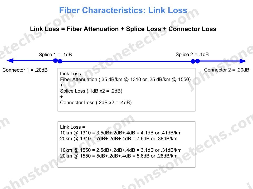
Fiber Attenuation vs Link Loss
Attenuation is a fiber property. Link loss is the whole problem.
Attenuation is the rate at which a fiber absorbs and scatters light as it travels — measured in dB per kilometer. It's a characteristic of the glass itself, and it doesn't change. Every reel of cable has an attenuation spec, and that number tells you what you're working with before you pull a single foot of it.
Link loss is the number that actually matters when you're testing. It's everything between your connectors: the fiber's attenuation over the full run, plus every splice along the way, plus the connectors at each end. That's the real insertion loss you're measuring when you put an OLTS on the link.
The reason this distinction matters in the field: if a link is failing its loss budget, knowing which piece is the problem tells you where to look. The fiber's attenuation is baked in — you can't change it. But a bad splice or a dirty connector is fixable, and you'll find it if you know what you're looking at.
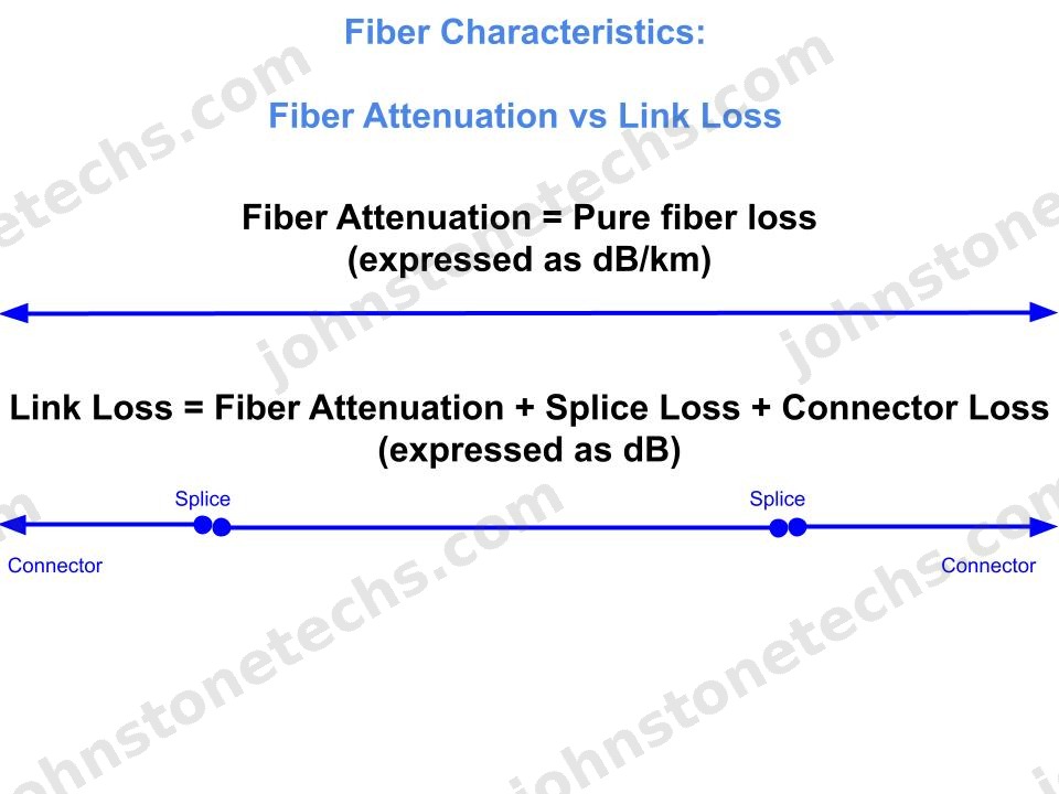
Fiber Attenuation — Reading the Specs
The number on the reel and the number in the ground are different questions.
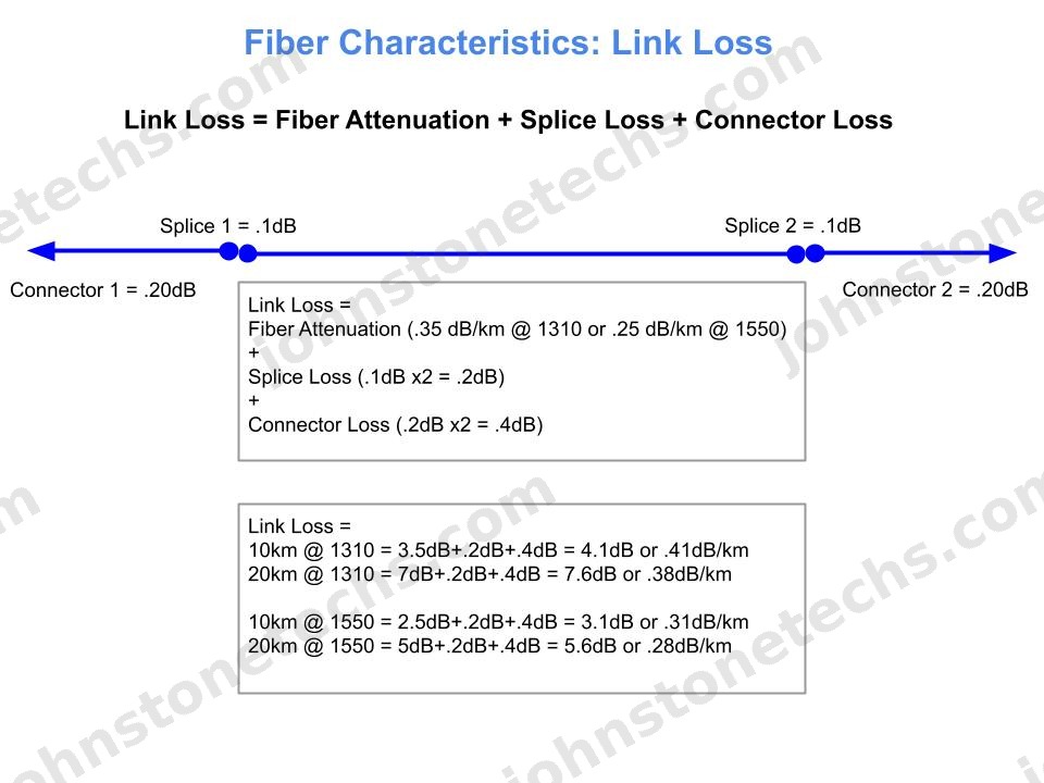
Every single-mode fiber has two published attenuation specs: one at 1310 nm and one at 1550 nm. Standard G.652D single-mode cable runs around 0.35 dB/km at 1310 and 0.25 dB/km at 1550. Those are the ceiling numbers from the manufacturer — most cable will beat them. But they're the ones you plan against when you're building a loss budget before the job.
Carriers have their own layer on top of that. A Verizon ODN table, for example, breaks the network into segments — feeder, distribution, drop — and sets an insertion loss limit for each. Those limits account for fiber attenuation, splices, connectors, and splitters all together. When you're doing acceptance testing on an FTTH build, those are the numbers you're proving against, not just the fiber manufacturer's spec.
If you're ever pulling cable for a job and you don't have the spec sheet in hand, get it before you place the order. The difference between a G.652D reel and a G.657A2 reel won't matter on a short run. On a long haul or a tight budget, it will.
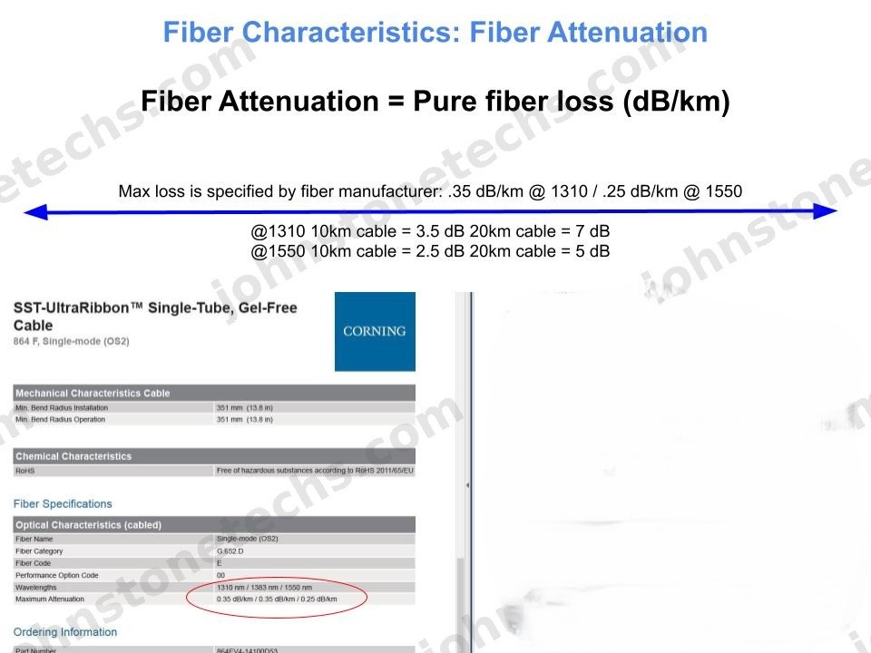
Reading an OLTS Results Report — FastReporter
Here's what a passing set of OLTS results actually looks like.
The FastReporter output shows you bidirectional loss at two wavelengths — 1310 nm and 1550 nm — with one pass in each direction on the same link. The A→Z and Z→A rows aren't redundant. Testing in both directions catches things a single-direction pass will miss: connector end-face offsets, splices where the fiber geometry isn't perfectly matched, and directional anomalies that only show up from one end.
The ORL column — optical return loss — is the measurement of how much light is reflecting back toward the source. High ORL is good. If that number drops too low, you've got a reflective event somewhere on the link: most likely a dirty or damaged connector, or an air gap at a mechanical splice. ORL failures are common on links that look fine on loss alone, which is why you always want it in the report.
A completed FastReporter set for carrier acceptance should show both wavelengths, both directions, ORL, and fiber length. If any of those are missing when you submit the test record, it's coming back to you.
.jpg)
OLTS Results in a Fiber Characterization Template
Raw test data is only as useful as the record it ends up in.
When you run OLTS on a link, the test equipment captures the numbers. What you do with those numbers after that determines whether you have documentation or just screenshots in a camera roll. A fiber characterization template gives every span a consistent home: fiber ID, wavelength, A→Z loss, Z→A loss, the bidirectional average, ORL, and a pass/fail against the budget.
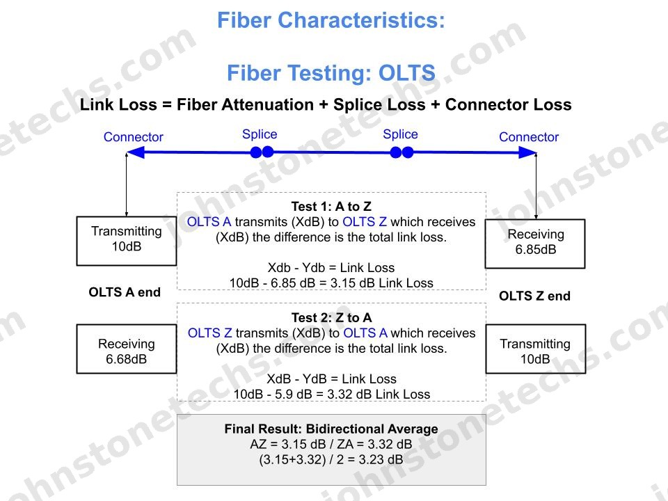
The bidirectional average is the number you submit. You run A→Z, run Z→A, add them, divide by two. That average removes the directional bias from connector offsets and gives you the actual link loss. It's what TIA-568 calls for and what most carriers require for acceptance. The template shown here makes that calculation explicit so there's no question how the number was derived.
If you're working a multi-span project — a feeder route, a distribution build, anything with more than a handful of fibers — a structured record like this is the difference between a clean handoff and a mess of paperwork at closeout. Build the template into the job from day one.
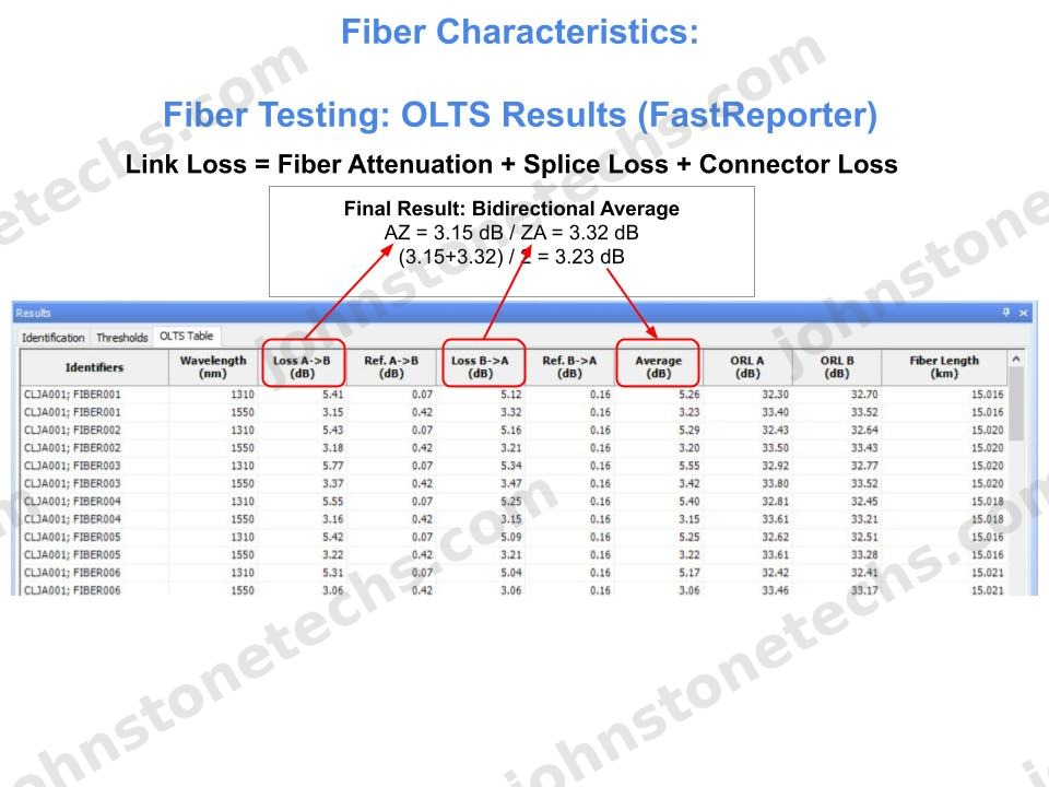
OLTS Bidirectional Test Methodology
Why you always test in both directions.
An OLTS measures end-to-end insertion loss by transmitting from one unit and reading at the other. Simple enough. The reason you run it twice — A→Z and then Z→A — is that connector geometry isn't perfect. The cores of two fibers at a mated pair aren't always centered exactly the same way, and the loss you see depends on which direction the light is traveling through the connection. A single-direction pass can show you 0.4 dB. Flip it and you might get 0.9 dB. The real number is the average of the two.
It's not just about connectors. Bidirectional testing also catches non-reciprocal events — things that only show up from one direction, which can point you toward a specific type of fault that's worth investigating before you put the link in service.
The method is straightforward: run A→Z at both wavelengths, have the far-end tech run Z→A, average the pairs. Most OLTS equipment automates this with a handshake between units. The output is a single bidirectional average per wavelength per span — the number that goes in the record, the number that gets submitted for acceptance.
Calculating Link Loss — Imperial Units
Do the math before you pull the cable.
A loss budget calculation tells you the maximum insertion loss you can expect on a link given its length, splice count, and connector count. You do this before the job so you know whether your link design is viable. You do it again after testing to know whether the numbers you measured are where they should be.
The formula is straightforward. Take the link distance in kilofeet, multiply by the loss coefficient for your fiber (typically around 1.1 dB/kft at 1310 nm for standard single-mode), then add your splice losses and connector losses on top. Use 0.1 dB per splice as a reasonable budget value for fusion splices. Connectors typically run 0.3–0.5 dB each depending on quality and cleanliness.
That total is your expected link loss. Compare it against your equipment's optical budget — transmit power minus receiver sensitivity — and you want a few dB of margin left over. If the math is tight on paper, it'll be tight in the field, and the first dirty connector or mediocre splice will put you over. Build in margin while you're still at the design stage.
Calculating Link Loss — Metric Units
Same calculation, metric units.
The link loss formula is the same regardless of what unit system you're working in. Distance times the fiber's attenuation coefficient, plus splice losses, plus connector losses, equals your expected end-to-end insertion loss. In metric the attenuation coefficient runs about 0.35 dB/km at 1310 nm and 0.25 dB/km at 1550 nm for standard G.652D single-mode — those are the manufacturer ceiling values, and real cable usually beats them.
If you're working off carrier specs or ITU documentation, you'll be in kilometers. If you're on a domestic OSP job in the US, you're probably working in feet and kilofeet. Either way, the calculation is the same and the pass/fail margin question is the same: does your expected loss leave enough headroom for the link to perform reliably over its life?
Run the numbers at both wavelengths. 1310 and 1550 behave differently, and some equipment is more sensitive at one than the other. A link that's comfortable at 1310 can be tight at 1550. If the carrier or the engineer specifies a loss limit, that limit applies at both wavelengths.