
Chromatic Dispersion is the calmer cousin of PMD. It doesn’t move around. It doesn’t change with the weather. Once a fiber is in the ground, its dispersion is a fixed number you can measure once and trust for the life of the cable. That makes it easier to test than PMD. It also makes it harder to fix, because there is nothing you can do to the glass to change it.
This is the CD deep dive. If you’re new to dispersion testing, start with the CD and PMD overview. If you’re testing a link that needs both, also read the PMD deep dive. This article covers what CD actually is, why different fiber types have different dispersion behavior, how it’s tested in the field, and how it’s dealt with at each layer of the network.
What CD actually is
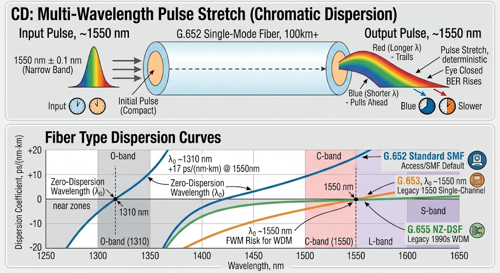
Your transmitter isn’t a perfect single-color laser. Even a good DFB laser puts out a narrow band of wavelengths, not a single wavelength. The blue end of that band travels through the fiber at one speed. The red end travels at a slightly different speed. Over a short span this makes no visible difference. Over hundreds of kilometers, the fastest wavelengths pull ahead of the slowest, and the pulse arrives at the far end smeared out in time.
That smear is chromatic dispersion. It’s measured in picoseconds per nanometer per kilometer, or ps/(nm·km). One ps/(nm·km) means: for every nanometer of wavelength spread in your source, and for every kilometer of fiber, you accumulate one picosecond of pulse spreading. Multiply your source’s spectral width by the span length, and you have your total accumulated dispersion in ps/nm.
That number then gets compared to the CD tolerance of your receiver. If it’s under the receiver’s budget, you’re fine. If it’s over, the pulse is spreading enough to close the eye.
Where the fiber’s dispersion comes from
Fibers aren’t all the same. What you’re measuring on any given span depends on how the fiber itself was engineered at the factory. Two properties combine to give a fiber its dispersion curve:
Material dispersion. Silica glass has an intrinsic wavelength-dependent refractive index. This is a property of the material and nobody can change it.
Waveguide dispersion. The way the refractive index is profiled between core and cladding affects how different wavelengths propagate. This is engineered at the preform stage and it’s the knob the fiber designer turns.
The combination determines the shape of the dispersion curve and, most importantly, where the curve crosses zero. This is called the zero-dispersion wavelength, or λ0.
The three fiber types you’ll see on real installs:
G.652: Standard Single-Mode Fiber
The workhorse. Engineered to have λ0 near 1310 nm. When you’re transmitting at 1310 nm, dispersion is near zero and you barely have to think about CD. When you’re transmitting in the C-band around 1550 nm (which is most modern long-haul and DWDM), CD is around +16 to +18 ps/(nm·km). Positive and not negligible.
This is what you’ll find in most access networks, most enterprise builds, and a lot of legacy long-haul plant. If someone says “single-mode fiber” without qualifying, they usually mean G.652.
G.653: Dispersion-Shifted Fiber (DSF)
Engineered with a modified waveguide dispersion to push λ0 from 1310 nm down into the 1550 nm window. When first developed, this seemed like a great idea: run at 1550 nm (lower loss than 1310) with near-zero CD. Then DWDM arrived. Running multiple wavelengths through a fiber with near-zero dispersion turned out to cause severe non-linear penalties, especially Four-Wave Mixing. G.653 largely fell out of favor for new builds. You’ll still find it on legacy long-haul that predates the DWDM era.
G.655: Non-Zero Dispersion-Shifted Fiber (NZ-DSF)
Engineered as a compromise after the G.653 lesson. λ0 is pushed near but not into the C-band. There’s enough dispersion in the working window (typically 2 to 6 ps/(nm·km) at 1550 nm) to suppress non-linear effects, but not so much that you need heavy compensation. Common on 1990s-era carrier long-haul builds.
Modern deployments have largely moved back to G.652 with coherent transceivers that handle CD in the receiver DSP, but G.655 is still in the ground on a lot of routes.
There are others (G.654, G.656, G.657), but these three cover the vast majority of what you’ll test.
Why CD is not like PMD
Two important differences from PMD, and getting them straight will save you time on real jobs.
CD is deterministic. Test the span today, test it tomorrow, test it a year from now. You get the same number every time within test-set tolerance. There’s no averaging over samples. There’s no statistical estimate. One test gives you the answer.
CD is a property of the fiber, not the deployment. Cable ties, splice tray dressing, aerial vibration, temperature swings — none of it affects CD in any meaningful way. If you walk the route and re-dress every splice enclosure, PMD may drop dramatically. CD will not budge.
This is why fixing CD failures is a different problem than fixing PMD failures. You can’t fix CD by fixing the plant.
How CD is tested
CD test sets are dual-ended. You need a source at one end and an analyzer at the other, coordinated on the same wavelength plan. Two common measurement methods:
Phase Shift Method
The most common approach in modern field CD analyzers. Modulate the source at a fixed RF frequency, launch across multiple wavelengths in sequence, and at the far end measure the RF phase shift of the received signal at each wavelength. The rate of change of phase with wavelength gives you the group delay, and the derivative of that gives you dispersion. The instrument does the math and reports back a ps/(nm·km) coefficient and a curve.
Differential Phase Shift and Time of Flight
Variations on the same idea. Time of Flight was more common on older instruments and directly measures the arrival time of pulses at different wavelengths. Both are still in use, but Phase Shift is what you’ll see on most modern gear.
The test itself takes 30 seconds to a few minutes per span once you’re set up. Like PMD, setup is where the time goes. Confirming both ends are on the same instrument settings, the same wavelength range, and the same reference cable takes longer than the measurement.
Most modern combined CD/PMD analyzers (EXFO FTB-5800, Viavi ODM in the T-BERD/MTS-8000 platform, Anritsu Network Master Pro with the CD/PMD module) can run both tests in the same setup, so you’re not tearing down and re-hooking between them.
Reading a CD test result
A CD analyzer will typically give you something like:
Span length:             24.6 km
Zero-dispersion (λ0):    1312 nm
Slope at λ0:            0.089 ps/(nm²·km)
Dispersion @ 1550 nm:    17.2 ps/(nm·km)
Total accumulated CD:    423 ps/nm at 1550 nm
Fiber type (estimated):  G.652
Example readout — field names, layout, and values vary by analyzer.
The two numbers that matter most on an acceptance report:
Dispersion coefficient at the working wavelength. Confirms the fiber type and gives you a per-km value.
Total accumulated dispersion for the span. This is what gets compared to the receiver’s CD tolerance. If the receiver is spec’d to tolerate 1,000 ps/nm, and your span comes in at 423 ps/nm, you’re comfortably inside budget.
Typical CD tolerances by bit rate:
| Bit rate | Modulation | Typical CD tolerance |
|---|---|---|
| 2.5G | NRZ direct detect | ~16,000 ps/nm |
| 10G | NRZ direct detect | 1,000 to 1,500 ps/nm |
| 40G | Various | 300 to 500 ps/nm |
| 100G coherent | DP-QPSK | 50,000+ ps/nm (DSP-managed) |
| 400G coherent | Various | Similar, DSP-managed |
Typical values for orientation — always confirm against the actual transceiver spec sheet.
Notice the pattern. Direct-detect systems get tighter as bit rates go up. Coherent systems break the pattern entirely because the DSP handles it. This is the single biggest thing to know about modern CD handling.
What can be done about CD
Unlike PMD, you cannot fix CD by walking the route. The intervention happens somewhere in the transmission chain, not at the fiber. There are four layers where CD gets managed, and the answer for any given circuit depends on what generation of gear it’s running on.
1. At the fiber itself
You can’t change it. What you can do is pick the right fiber for the wavelength you’re transmitting at. This is a design-time decision. If a new build is being engineered, G.652 with coherent transceivers is the modern default. If a route is being lit for the first time on legacy G.653 or G.655, the transport team factors that into the compensation plan.
2. In-line optical compensation
Dispersion Compensating Fiber (DCF) is a spool of specialized fiber with a large negative dispersion coefficient, typically -80 to -120 ps/(nm·km). It gets spliced into the mid-stage of an EDFA amplifier. The negative dispersion cancels the positive dispersion the signal accumulated on the previous span.
Chirped Fiber Bragg Gratings (FBGs) do the same job with a compact passive device that reflects different wavelengths at different physical depths, unwinding the pulse spreading with less insertion loss and less latency than a DCF spool.
You’ll encounter both in existing plant. You won’t often see them on new builds because modern coherent transceivers make them unnecessary and even counterproductive.
3. At the transmitter
Laser pre-chirping applies a controlled frequency sweep to the pulse at the transmitter, so the pulse initially compresses as it hits the fiber before starting to spread. Used on some 10G and 40G direct-detect systems.
Tx-EDC (Transmit Electronic Dispersion Compensation) applies inverse phase profiles in the transmitter DSP before the digital-to-analog conversion. Found on advanced direct-detect transceivers.
Both are ways of pre-loading the signal so that after fiber dispersion, the pulse arrives correctly shaped.
4. At the receiver
This is where modern coherent networks handle CD, and it’s the reason inline compensation has largely gone away on new builds.
A coherent receiver captures both the amplitude and phase of the incoming signal using a local oscillator laser. Its DSP then applies the exact mathematical inverse of the fiber’s dispersion transfer function using FIR or FFT-based frequency-domain equalization. Because the receiver sees the full complex field, it can undo essentially any amount of dispersion within its processing budget. 100G and 400G coherent systems routinely handle 50,000+ ps/nm without inline compensation.
Why modern networks skip inline compensation
If DCF and FBGs work fine and coherent DSP works fine, why not use both? Because inline compensation adds insertion loss, adds latency, and encourages non-linear penalties.
The physics: high-power WDM channels traveling through a fiber with low local dispersion mix with each other and generate spurious signals. This is Four-Wave Mixing. The lower the local dispersion, the worse it gets. Cross-Phase Modulation is a related effect. Both degrade signal quality in ways that DSP can’t fully undo.
An uncompensated link (all positive dispersion accumulating across the whole route, corrected only at the receiver) has higher local dispersion at every point along the run, which suppresses non-linear mixing. It also has lower total loss (no DCF insertion) and lower latency (no DCF or FBG delay). Modern coherent networks are designed to lean into all three of these advantages.
The short version: on modern 100G+ coherent networks, don’t be surprised if there’s no inline compensation on the route and the DSP is doing all the CD work. That’s the current best practice, not a shortcut.
On older direct-detect systems and existing plant with DCF already installed, the older approaches are still in service and still work.
What CD is not
CD is not loss. Fixing loss won’t drop CD. Fixing CD won’t drop loss.
CD is not PMD. Both broaden the pulse, but CD is deterministic and PMD is statistical. CD is set by the fiber design and PMD is set by the fiber plus every stress in the deployment. If your circuit needs full acceptance testing at high bit rates, you test for both separately. See the PMD deep dive for the other half.
Related tools and articles
- CD and PMD Testing Overview — start here for the big picture.
- PMD Testing Deep Dive — the PMD companion to this article.
- Fiber Loss Calculator — for the separate loss-budget half of acceptance testing.
- Fiber Trace Analyzer — for reading OTDR traces on the same job.